Mathematics#
Numpy Arrays#
import numpy as np
import matplotlib.pyplot as plt
l = [0.0,1.0,2.0]
a = np.array(l)
print(l)
print(a)
print(a.mean())
print(type(a))
print(a.dtype)
print(a.shape)
a = np.zeros([3,5])
print(a)
print(a.shape)
a[0,1] = 75
print(a)
a = np.ones([2,3])
print(a)
a = np.array([[1,2,3], [3,4,5]])
print(a)
a = np.array([1,2,3])
b = np.array([4,5,6])
c = np.vstack([a,b])
print(c)
np.hstack([a,b])
np.shape(c)
x = np.arange(1,100,0.3)
y = np.linspace(1,101,400)
[0.0, 1.0, 2.0]
[0. 1. 2.]
1.0
<class 'numpy.ndarray'>
float64
(3,)
[[0. 0. 0. 0. 0.]
 [0. 0. 0. 0. 0.]
 [0. 0. 0. 0. 0.]]
(3, 5)
[[ 0. 75.  0.  0.  0.]
 [ 0.  0.  0.  0.  0.]
 [ 0.  0.  0.  0.  0.]]
[[1. 1. 1.]
 [1. 1. 1.]]
[[1 2 3]
 [3 4 5]]
[[1 2 3]
 [4 5 6]]
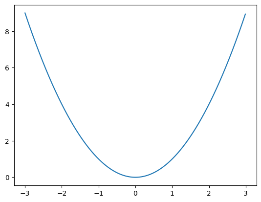
x = np.arange(-3,3,0.01)
y = x**2
plt.plot(x,y)
plt.show()
print(c)
print(c[:,:-1])

data_set = np.array([
    [0,1,2,3],
    [2,4,6,8],
    [3,3,3,3],
    [4,2,1,3],
    [3,3,1,2]
])
split = 3
train, test = data_set[:split, :], data_set[split:,:]
print(train)
print(test)
[[1 2 3]
 [4 5 6]]
[[1 2]
 [4 5]]
[[0 1 2 3]
 [2 4 6 8]
 [3 3 3 3]]
[[4 2 1 3]
 [3 3 1 2]]
data_set=data_set.reshape((1,20))
print(data_set)
[[0 1 2 3 2 4 6 8 3 3 3 3 4 2 1 3 3 3 1 2]]
data_set = np.array([
    [0,1,2,3],
    [2,4,6,8],
    [3,3,3,3],
    [4,2,1,3],
    [3,3,1,2]
])
sum_of_rows = np.sum(data_set, 0)
sum_of_columns = np.sum(data_set, 1)
print(sum_of_rows)
[12 13 13 19]
data_set[:,1] = data_set[:,1] - 1
print(data_set)
[[0 0 2 3]
 [2 3 6 8]
 [3 2 3 3]
 [4 1 1 3]
 [3 2 1 2]]
print(data_set/(data_set+1))
[[0.         0.         0.66666667 0.75      ]
 [0.66666667 0.75       0.85714286 0.88888889]
 [0.75       0.66666667 0.75       0.75      ]
 [0.8        0.5        0.5        0.75      ]
 [0.75       0.66666667 0.5        0.66666667]]
If \(a = (a_1, a_2, \ldots, a_n)\), \(b = (b_1, b_2, \ldots, b_n)\) then \(a\cdot b = a_1b_1 + a_2b_2 +\cdots + a_nb_n\)
a = np.array([2,3])
b = np.array([1,7])
print(a.dot(b))
23
print(a)
cons = 4
print(cons*a)
[2 3]
[ 8 12]
\(a = (a_1, a_2,\ldots, a_n)\)
\(||a||_1 = |a_1|+|a_2|+\cdots +|a_n|\)
\(||a||_2 = \sqrt{a_1^2+a_2^2+\cdots + a_n^2}\)
print(a)
l1_of_a = np.linalg.norm(a, 1)
print(l1_of_a)
l2_of_a = np.linalg.norm(a)
print(l2_of_a)
[2 3]
5.0
3.605551275463989
print(data_set)
print(data_set.T)
print(data_set.T.dot(data_set))
print(data_set.T@data_set)
[[0 0 2 3]
 [2 3 6 8]
 [3 2 3 3]
 [4 1 1 3]
 [3 2 1 2]]
[[0 2 3 4 3]
 [0 3 2 1 2]
 [2 6 3 1 1]
 [3 8 3 3 2]]
[[38 22 28 43]
 [22 18 27 37]
 [28 27 51 68]
 [43 37 68 95]]
[[38 22 28 43]
 [22 18 27 37]
 [28 27 51 68]
 [43 37 68 95]]
u = np.array([2,0]).reshape(2,1)
np.sqrt(u.T.dot(u))
array([[2.]])
Length of the projection of \(u\) on \(v\) is \(\dfrac{u\cdot v}{||v||}\)
Projection of \(u\) on \(v\) is \(\left(\dfrac{u\cdot v}{||v||}\right) \dfrac{v}{||v||}\)
u = np.array([2,0])
v = np.array([3,3])

norm_v = np.linalg.norm(v)

length_p_u_on_v = (u.dot(v/norm_v))
print(length_p_u_on_v)
print(length_p_u_on_v*(v/norm_v))
1.4142135623730951
[1. 1.]
u = np.array([1,1,0])
v = np.array([0,1,1])
norm_v = np.linalg.norm(v)

length_p_u_on_v = (u.dot(v/norm_v))
print(length_p_u_on_v)
print(length_p_u_on_v*(v/norm_v))
0.7071067811865475
[0.  0.5 0.5]
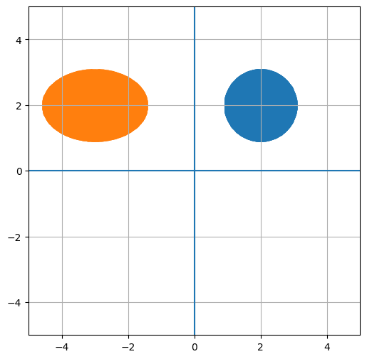
Matrix Multiplication to transform the data#
c = np.array([2,2])
r = 1
inc = 0.01
x = np.arange(c[0]-r, c[0]+r, inc)
my_data = []
for val in x :
    ymin = c[1] - np.sqrt(r**2 - (val - c[0])**2 )
    ymax = c[1] + np.sqrt(r**2 - (val - c[0])**2 )
    rng = np.arange(ymin, ymax, inc)
    for yval in rng:
        my_data.append([val, yval])


my_data = np.array(my_data)
T_mat = np.array([[-1.5,0],[0,1]])
T_data = (T_mat@(my_data.T)).T
print(my_data.shape)
fig, ax = plt.subplots(figsize=(6,6))
ax.scatter(my_data[:,0], my_data[:,1])
ax.scatter(T_data[:,0], T_data[:,1])
plt.axhline()
plt.axvline()
plt.xlim(-5,5)
plt.ylim(-5,5)
plt.grid()
plt.show()
(31497, 2)
T_mat = np.array([[-1,0],[0,-1]])
print(T_mat)
print(T_mat@np.array([[1,0], [0,1]]))
[[-1  0]
 [ 0 -1]]
[[-1  0]
 [ 0 -1]]
print(np.eye(3))
[[1. 0. 0.]
 [0. 1. 0.]
 [0. 0. 1.]]
m = np.array([ [1,2,3],
               [4,5,6],
               [7,8,9]
])
upper_m = np.triu(m)
print(upper_m)
lower_m = np.tril(m)
print(lower_m)
[[1 2 3]
 [0 5 6]
 [0 0 9]]
[[1 0 0]
 [4 5 0]
 [7 8 9]]
print(np.diag(m))
[1 5 9]
Orthogonal Matrix#
Matrices with orthogonal columns and are all of length one.
Q = np.array([[1,0],[0,-1]])
Q@(Q.T)
array([[1, 0],
       [0, 1]])
Inverse of a matrix#
a= np.array([[1,0], [-2,1]])
print(np.array([[1,0], [2,1]])@a)
[[1 0]
 [0 1]]
print(np.linalg.inv(np.array([[1,0], [-2,1]])))
[[ 1. -0.]
 [ 2.  1.]]
Determinant#
print(np.linalg.det(np.array([[1,0], [-2,1]])))
1.0
Rank#
print(np.linalg.matrix_rank(np.array([[1,2,3], [0,1, 0]])))
2
Trace#
Trace of a matrix is the sum of its diagonal
A = np.array([[1, 2, 3], [4, 5, 6], [7, 8, 9]])
print(A)
# calculate trace
b = np.trace(A)
print(b)
[[1 2 3]
 [4 5 6]
 [7 8 9]]
15
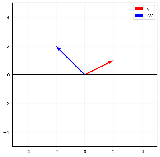
Plotting a vector v and a vector Av#
# Change A and v and see what happens to Av
v = np.array([[2],[1]])
A = np.array([[-1,0],[0,2]])
Av = A@v
fig, ax = plt.subplots(figsize=(6,6))

ax.quiver(0,0, v[0,0], v[1,0], angles='xy', scale_units='xy', scale=1, color="r", label="$v$")
ax.quiver(0,0, Av[0,0], Av[1,0], angles='xy', scale_units='xy', scale=1, color="b", label="$Av$")
plt.axhline(color = 'k')
plt.axvline(color = 'k')
plt.ylim(-5,5)
plt.xlim(-5,5)
plt.grid()
plt.legend()
plt.show()
More Array Methods#
a = np.array([4, 3, 2, 1])
a
array([4, 3, 2, 1])
a.sort()              # Sorts a in place
a
array([1, 2, 3, 4])
a.max() # Max
4
a.argmax() # Returns the index of the maximal element
3
a.cumsum() # Cumulative sum of the elements of a
array([ 1, 3, 6, 10])
a.cumprod() # Cumulative product of the elements of a
array([ 1, 2, 6, 24])
a.var() # Variance
1.25
a.std() # Standard deviation
1.118033988749895
z = np.linspace(2, 10, 6)
z
array([ 2. , 3.6, 5.2, 6.8, 8.4, 10. ])
# If z is a nondecreasing array, then z.searchsorted(a) returns the index of the first element of z that is >= a
z.searchsorted(4)
2
a = np.random.randn(3) # Generate a random array of size 3 from N(0,1) distribution
a
array([-0.84580538, -0.16634285, 0.01221481])
Applying functions on arrays#
z = np.array([0, 1, np.pi/2, np.pi])
print(np.sin(z))
print(np.round(np.sin(z),2))
[0.00000000e+00 8.41470985e-01 1.00000000e+00 1.22464680e-16]
[0.   0.84 1.   0.  ]
Evaluating the value of \(\frac{1}{\sqrt{2\pi}}e^{-\frac{z^2}{2}}\) at \(z =1, 2\) and \(3\).
z = np.array([1,2,3])
(1 / np.sqrt(2 * np.pi)) * np.exp(- 0.5 * (z**2))
array([0.24197072, 0.05399097, 0.00443185])
Not all user-defined functions will act element-wise.
def f(x):
    if x > 2:
        return 1
    else:
        return 0
# Now try f(z) and you will get an error
# Instead of writing the loop and applying f to each element of z, here is an alternative
np.where(z > 2, 1, 0)
array([0, 0, 1])
# Alternatively, you can also use np.vectorize to vectorize a given function
f = np.vectorize(f)
f(z)
array([0, 0, 1])
Comparing arrays#
z = np.array([2, 3])
y = np.array([2, 3])
z == y
array([ True, True])
y[0] = 9
print(y)
print(z)
z == y
[9 3]
[2 3]
array([False, True])
z != y
array([ True, False])
z = np.linspace(0, 10, 5)
print(z)
print(z > 3)
[ 0.   2.5  5.   7.5 10. ]
[False False  True  True  True]
Subsetting a vector using a condition
print(z)
z[z > 3]
[ 0. 2.5 5. 7.5 10. ]
array([ 5. , 7.5, 10. ])
Solving for \(x\): \(Ax = b\)
A = np.array([[3,2,0],[1,-1,0],[0,5,1]])
b = np.array([2,4,-1])
x = np.linalg.solve(A,b)
print(x)
print(A.dot(x))
[ 2. -2.  9.]
[ 2.  4. -1.]
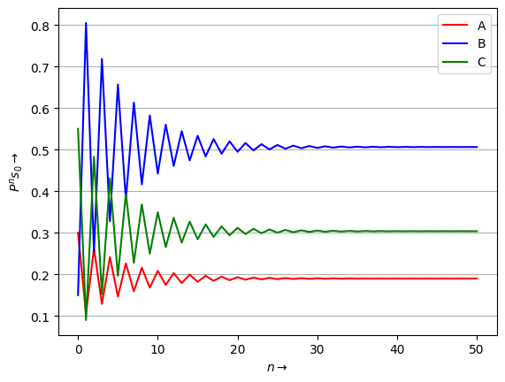
EigenValue and Eigenvectors: \(Av = \lambda v\)
import pandas as pd

s0 = np.array([0.3,0.15,0.55])
P = np.array([[0.2,0.3,0],[0.8,0.1,1],[0,0.6,0]])
s1 = P@s0
n= 50
data = []
data.append(list(s0))
s= s0
for i in range(n):
    s = P@s
    data.append(list(s))


df = pd.DataFrame(data)
df.columns =["A","B","C"]
df
ax = plt.axes()
ax.yaxis.grid(True)
plt.plot(range(n+1), df["A"], c = "r", label='A')
plt.plot(range(n+1), df["B"], c = "b", label='B')
plt.plot(range(n+1), df["C"], c = "g", label ='C')
plt.xlabel(r"$n\rightarrow$")
plt.ylabel(r"$P^ns_0\rightarrow$")
plt.legend()
plt.show()
df.tail()
| A | B | C | |
|---|---|---|---|
| 46 | 0.189912 | 0.506196 | 0.303892 |
| 47 | 0.189841 | 0.506441 | 0.303717 |
| 48 | 0.189901 | 0.506235 | 0.303865 |
| 49 | 0.189850 | 0.506409 | 0.303741 |
| 50 | 0.189893 | 0.506262 | 0.303845 |
Let \(V\) denote the Eigenvalues and \(E\) be the matrix of Eigenvectors associated with matrix \(P\).
V, E = np.linalg.eig(P)

print('V={}'.format(V))

print('E={}'.format(E))

print('inv(E)PE={}'.format(np.linalg.inv(E)@P@E))

print('E diag(V)inv(E)={}'.format(E@np.diag(V)@np.linalg.inv(E)))
V=[ 1.          0.14244289 -0.84244289]
E=[[-0.30612245  0.76925258  0.22822377]
 [-0.81632653 -0.14758652 -0.79303414]
 [-0.48979592 -0.62166606  0.56481038]]
inv(E)PE=[[ 1.00000000e+00 -2.22044605e-16 -5.55111512e-17]
 [-4.16333634e-17  1.42442890e-01 -6.93889390e-17]
 [-3.33066907e-16  5.55111512e-17 -8.42442890e-01]]
E diag(V)inv(E)=[[2.00000000e-01 3.00000000e-01 8.90563616e-17]
 [8.00000000e-01 1.00000000e-01 1.00000000e+00]
 [6.60698968e-17 6.00000000e-01 6.14650667e-17]]
\(P = EVE^{-1}\)
\(P^2 =EVE^{-1}EVE^{-1} = EV^2E^{-1} \)
\(P^n = EV^nE^{-1}\)
print(P@P@P@P@P)
print(E@((np.diag(V)) **5)@np.linalg.inv(E))
[[0.14456 0.24897 0.1197 ]
 [0.66392 0.30097 0.7501 ]
 [0.19152 0.45006 0.1302 ]]
[[0.14456 0.24897 0.1197 ]
 [0.66392 0.30097 0.7501 ]
 [0.19152 0.45006 0.1302 ]]
\(\displaystyle\left( \frac{y^Tx}{||x||}\right)\left( \frac{x}{||x||}\right)\)
\((y-X\beta)^T(X\beta) = 0\)
Here \(X\) is \(m \times k\), \(y\) is \(m \times 1\), \(\beta\) is \(k \times 1\)
\((y^T-\beta^TX^T)(X\beta) = 0\)
\(y^TX = \beta^TX^TX\)
\((X^TX)^{-1} X^{T}y = \beta\)
from sympy import *
from sympy.abc import a, m
t, x, y, n, k = symbols('t x y n k')
f = Function('f g')
f = integrate(2-2*t,(t,0,y))
solve(Eq(f, x),y)[0]
g = integrate(t*(2-2*t),(t,0,y))
g.subs({y:solve(Eq(f, x),y)[0]})
limit(1/log(x) - 1/(x-1),x,1)
Sum( (1/k)*((-1)**(k+1)),(k,1,oo))
limit_seq(Sum(k**2 * Sum(2**m/m, (m, 1, k)), (k, 1, n)) / (2**n*n), n)
expr = log(x)
expr.series(x, 1, 8)
g = atan((3*x-x**3)/(1-3*(x**2)))
g
diff(g,x)
f = atan((2*x)/(1-(x**2)))
f
diff(f,x)
simplify(diff(g,x)/diff(f,x))
sigma, mu, x, y, p, m, s, z, Q, omg1, omg2, t = symbols('sigma μ x y p m s z Q 𝜔1 𝜔2 t')
Phi = Function('Φ')
l = Function('𝑣𝑙')
u = Function('𝑣𝑢')
sigma
Phi = (1+erf(x/(sqrt(2))))/2
diff(Phi,x)
integrate((1/sqrt(2*pi))*exp(1)**(-z**2/2),(z,-oo,x))
Phi.evalf(subs={x:1}) - Phi.evalf(subs={x:0})
f = 2-2*t
F = integrate(f, (t,0,z))
solve(F-x,z)[0]
sol = solveset(F-x,z, domain=Interval(0, 1))
print(sol)
sol.evalf(subs = {x:0.8})
Intersection({1 - sqrt(1 - x), sqrt(1 - x) + 1}, Interval(0, 1))
integrate(f*t, (t,0,solve(F-x,z)[0]))/integrate(f*t, (t,0,1))
z=Symbol('z', positive = True)

f = 2-2*t
F = integrate(f, (t,0,z))
g = integrate(f*t, (t,0,solve(F-x,z)[0]))/integrate(f*t, (t,0,1))
g
2*integrate(x-g, (x,0,1))
f= Rational(1,5)
f
F = integrate(f, (t,0,z))
F
solve(F-x,z)[0]
g = integrate(f*t, (t,0,solve(F-x,z)[0]))/integrate(f*t, (t,0,5))
g
2*integrate(x-g, (x,0,1))
f = Rational(2,25)*t
f
F = integrate(f, (t,0,z))
F
solve(F-x,z)
[-5*sqrt(x), 5*sqrt(x)]
g = integrate(f*t, (t,0,solve(F-x,z)[1]))/integrate(f*t, (t,0,5))
g
2*integrate(x-g, (x,0,1))
phi = Symbol('phi')
phi
diff(x**2 * y**3 * z, x, y,z)
f = Rational(1,2)*t
f
F = integrate(f, (t,0,z))
F
solve(F-x,z)[1]
g = integrate(f*t, (t,0,solve(F-x,z)[1]))/integrate(f*t, (t,0,2))
g
2*integrate(x-g, (x,0,1))
f = 2*t
f
F = integrate(f, (t,0,z))
F
solve(F-x,z)[0]
g = integrate(f*t, (t,0,solve(F-x,z)[0]))/integrate(f*t, (t,0,1))
g
2*integrate(x-g, (x,0,1))
f = (3*(t-1)**2)
f
F = integrate(f, (t,1,z))
F
solve(F-x,z)[0]
g = integrate(f*t, (t,1,solve(F-x,z)[0]))/integrate(f*t, (t,1,2))
g
2*integrate(x-g, (x,0,1))
Integral(floor(x), (x, 0, 0.5)).doit()
def f(x):
    return x**3 + 3*(x**2) - 24

def df(x):
    return 3*(x**2) + 6*x

def update_x(x):
    return x - f(x)/df(x)

x = 2.0
print(x, f(x))
n = 3
for i in range(3):
    x = update_x(x)
    print(x, f(x))
2.0 -4.0
2.1666666666666665 0.2546296296296262
2.157264957264957 0.0008388942896928597
2.157233777359778 9.208314111219806e-09
def f(x):
    return x**3 + 3*(x**2) - 24

def df(x):
    return 3*(x**2) + 6*x

def update_x(x):
    return x - f(x)/df(x)

x = 3.0
print(x, f(x))
n = 3
for i in range(3):
    x = update_x(x)
    print(x, f(x))
3.0 30.0
2.3333333333333335 5.037037037037042
2.167277167277167 0.2711675621460117
2.1572691132802224 0.0009507119028313582
from sympy import *
from sympy.abc import x
f = Function('f')
f = x**2 - 10
f
g = diff(f,x)
g
u = x - f/g
u
simplify(u)
x0 = 3
for i in range(4):
    x0 = u.evalf(subs = {x:x0})
    print(x0)
3.16666666666667
3.16228070175439
3.16227766016984
3.16227766016838
from sympy import *
from sympy.abc import x

f1 = Rational(1,6)*exp(-x)*(exp(3*x) + sin(3*x) + 5*cos(3*x))
simplify(f1.diff(x))
f2 = Rational(1,6)*exp(-x)*(exp(3*x) + 5*sin(3*x) + 5*cos(3*x))
simplify(f2.diff(x))
print(latex(f1))
\frac{\left(e^{3 x} + \sin{\left(3 x \right)} + 5 \cos{\left(3 x \right)}\right) e^{- x}}{6}
print(latex(f2))
\frac{\left(e^{3 x} + 5 \sin{\left(3 x \right)} + 5 \cos{\left(3 x \right)}\right) e^{- x}}{6}
print(latex(simplify(f1.diff(x))))
\frac{\left(e^{3 x} - 8 \sin{\left(3 x \right)} - \cos{\left(3 x \right)}\right) e^{- x}}{3}
simplify(f1.diff(x,x) + 2*f1.diff(x) + 10*f1)
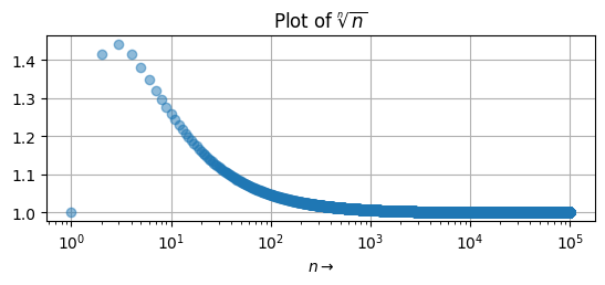
n=np.arange(1, 10**5)
fig = plt.figure()
ax = fig.add_subplot(2, 1, 1)
ax.set_xscale('log')
ax.plot(n, n**(1/n), 'o', alpha = 0.5)
ax.set_title('Plot of '+r'$\sqrt[n]{n}$')
ax.set_xlabel(r'$n\rightarrow$')
ax.grid()
plt.show()
from sympy import *
from sympy.abc import c, x
q1 = Rational(1,4)*(1-c)
q1
q2 = Rational(1,4)*(1-c)
q2
q = q1+ q2
q
p=1-q
p
f = 1-x
cs = simplify(integrate(f-p,(x,0,q)))
ps = simplify(integrate(p-c,(x,0,q)))
ps
g= Rational(1,2)*((1-c)**2)
simplify(g-ps-cs)