Statistics & Learning

Supervised Learning

Linear Regression

import numpy as np
import pandas as pd
import matplotlib.pyplot as plt

data = pd.read_csv('https://piazza.com/redirect/s3?bucket=uploads&prefix=paste%2Fi5t4zjz64oq3sl%2Fe69559fac1a2f68f704222629e603299bfa8aabfd88e81225e52e125484764a0%2Fdata1.txt', sep = ",", header=None)
data.columns = ["Pop", "Profit"]

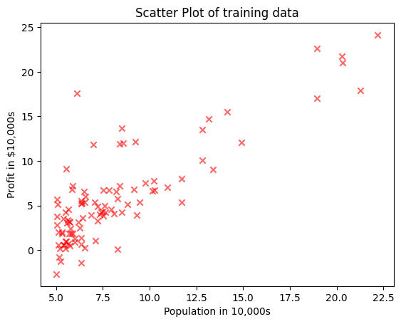
plt.scatter(data["Pop"], data["Profit"], marker = "x", alpha = 0.6, color = "r")
plt.xlabel("Population in 10,000s")
plt.ylabel("Profit in $10,000s")
plt.title("Scatter Plot of training data")
plt.show()

def normalEqn(X, y):
    return (np.linalg.inv(X.T@X) @  X.T@y)

X = pd.DataFrame(data["Pop"])
y = data["Profit"]
m = len(y)
constant = np.ones(m)
X.insert(0, "constant", constant)
b = normalEqn(X, y)
print("intercept =",b[0],", slope =", b[1])

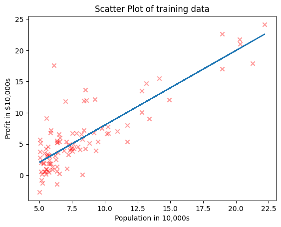
intercept = -3.89578087831185 , slope = 1.1930336441895941

plt.scatter(data["Pop"], data["Profit"], marker = "x", alpha = 0.4, color = "r")
plt.plot(data["Pop"], b[0] + b[1]*data["Pop"])
plt.xlabel("Population in 10,000s")
plt.ylabel("Profit in $10,000s")
plt.title("Scatter Plot of training data")
plt.show()

def cost(X, y, theta):
    m = len(y)
    J = (1/(2*m))*(((X@theta-y)**2).sum())
    return J

def gradientDescent(X, y, theta, alpha, iterations):
    m = len(y)
    J_history = np.zeros(iterations)
    for iter in range(iterations):
        theta = theta - (((alpha/m)*(X@theta - y).T@X).T)
        J_history[iter] = cost(X, y, theta)
    return theta, J_history

theta = np.zeros(2)
iterations = 1500
alpha = 0.02

print(cost(X,y, theta))

32.072733877455676

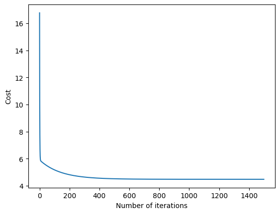
theta, J_history = gradientDescent(X, y, theta, alpha, iterations)
print("intercept =",theta[0],", slope =", theta[1])

intercept = -3.878137690865592 , slope = 1.191261194638165

plt.plot(range(iterations),J_history)
plt.xlabel('Number of iterations')
plt.ylabel('Cost')
plt.show()

from sklearn import linear_model
reg = linear_model.LinearRegression()
reg.fit(X.iloc[:,1:], y)
print("intercept =",reg.intercept_,", slope =", reg.coef_[0])

---------------------------------------------------------------------------
ModuleNotFoundError                       Traceback (most recent call last)
Cell In[12], line 1
----> 1 from sklearn import linear_model
      2 reg = linear_model.LinearRegression()
      3 reg.fit(X.iloc[:,1:], y)

ModuleNotFoundError: No module named 'sklearn'

data = pd.read_csv('https://piazza.com/redirect/s3?bucket=uploads&prefix=paste%2Fi5t4zjz64oq3sl%2Fc19f8051a03d4b73be5bb9a60ace1c2f24adba2947cc0028e0f184d5680d4d21%2Fdata2.txt', sep = ",", header=None)
data.columns = ["Size", "Bedrooms", "Price"]
data.head()

	Size	Bedrooms	Price
0	2104	3	399900
1	1600	3	329900
2	2400	3	369000
3	1416	2	232000
4	3000	4	539900

X = data.iloc[:,:-1]
y = data.iloc[:,2]
m = len(y)
def normalize(X):
    X_norm = (X - np.mean(X,0))/np.std(X,0)
    mu = np.mean(X,0)
    sigma = np.std(X,0)
    return X_norm, mu, sigma

X, mu, sigma = normalize(X)

one = np.ones((m,1))
X.insert(0, 'constant', one)

alpha = 0.1
iterations = 500
theta = np.zeros(3)
theta, J_history = gradientDescent(X, y, theta, alpha, iterations)

print(theta)

constant    340412.659574
Size        109447.796460
Bedrooms     -6578.354844
dtype: float64

print(normalEqn(X, y))

0    340412.659574
1    109447.796470
2     -6578.354854
dtype: float64

reg = linear_model.LinearRegression()
reg.fit(X.iloc[:,1:], y)
print(reg.intercept_, reg.coef_)

340412.6595744681 [109447.79646964  -6578.35485416]

# Predicting the price of the house with following features : size = 2000 sqft, number of bedrooms = 4
size = 2000
bedrooms = 4
normalized = (np.array([size, bedrooms]) - mu)/sigma
print("Predicted Price of house of size {} sq ft and number of bedrooms {} is around ${}".format(size, bedrooms, round(theta[0] + theta[1]*normalized[0] + theta[2]*normalized[1])))

Predicted Price of house of size 2000 sq ft and number of bedrooms 4 is around $333067

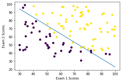
Logistic Regression

data = pd.read_csv('https://piazza.com/redirect/s3?bucket=uploads&prefix=paste%2Fi5t4zjz64oq3sl%2Fed7298995232c17a7f1bc50c9807cb7216337563e4a7c00bfcaa8f5d6bd32f02%2Fdata3.txt', sep = ",", header=None)
data.columns = ['Exam1', 'Exam2', 'Admit']

X = data.iloc[:,:2]
y = data.iloc[:,2]

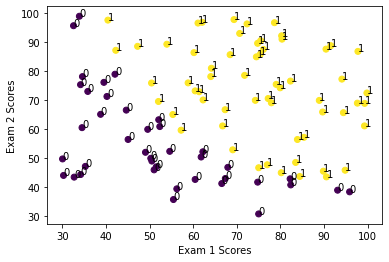
plt.scatter(X["Exam1"], X["Exam2"], c = y)
for i, label in enumerate(list(y)):
    plt.text(X["Exam1"][i], X["Exam2"][i],label)
plt.xlabel("Exam 1 Scores")
plt.ylabel("Exam 2 Scores")
plt.show()

from sklearn.linear_model import LogisticRegression
reg = LogisticRegression()
reg.fit(X,y)
print(reg.intercept_, reg.coef_)

[-25.05219314] [[0.20535491 0.2005838 ]]

t0 = reg.intercept_[0]
t1 = reg.coef_[0,0]
t2 = reg.coef_[0,1]

l = X['Exam1'].min()
u = X['Exam1'].max()
x1 = np.array([l, u])
x2 = (-t0/t2) - (t1/t2)*x1

plt.scatter(X["Exam1"], X["Exam2"], c = y)
plt.plot(x1, x2)
plt.xlabel("Exam 1 Scores")
plt.ylabel("Exam 2 Scores")
plt.show()

# Predicting the admission decision when scores of the student are : Score in Exam 1 = 80, Score in Exam 2 = 45
s1 = 80
s2 = 45
positive = t0 + t1*s1 + t2*s2 >= 0
if positive:
    print('Chances of admission are high.')
else:
    print('Admission is unlikely.')

Chances of admission are high.