Probability

Contents

Probability#

Discrete Random Variables#

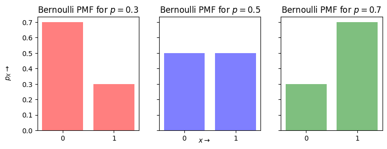
Bernoulli Random Variable#

import matplotlib.pyplot as plt
import numpy as np
from scipy.stats import binom

n=1
x = np.arange(0,n+1,1)
xs = [str(x[i]) for i in range(len(x))]
p = [0.3,0.5,0.7]
width = 0.35  # the width of the bars
cols = ['r', 'b', 'g']
fig, axs = plt.subplots(1, len(p), figsize=(3*len(p), 3), sharey=True)
for i in range(len(p)):
    axs[i].bar(xs, binom.pmf(x, n, p[i]), alpha=0.5, color=cols[i])
    axs[i].set_title('Bernoulli PMF for ' + r'$p={}$'.format(p[i]))
fig.text(0.5, 0.04, r'$x\rightarrow$', ha='center', va='center')
fig.text(0.06, 0.5, r'$p_X\rightarrow$', ha='center', va='center', rotation='vertical')

plt.show()

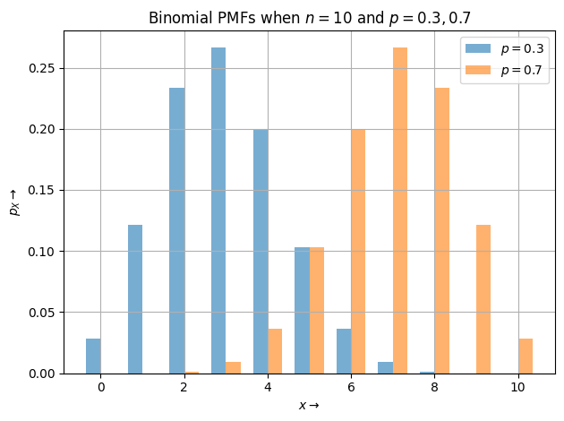
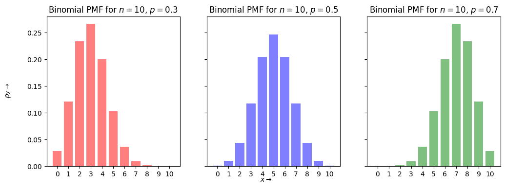
../_images/3361df94c2a9a1959bb487828c0b4838eb4d1fe97deba16557f75bfc4293ab23.png

Binomial Random Variable#

n=10
x = np.arange(0,11,1)
p1=0.3
p2=0.7
y1 = binom.pmf(x, n, p1)
y2 = binom.pmf(x, n, p2)

width = 0.35  # the width of the bars

fig, ax = plt.subplots()
ax.grid()
rects1 = ax.bar(x - width/2, y1, width, alpha = 0.6, label='$p={}$'.format(p1))
rects2 = ax.bar(x + width/2, y2, width, alpha = 0.6, label='$p={}$'.format(p2))

# Add some text for labels, title and custom x-axis tick labels, etc.
ax.set_ylabel(r'$p_X\rightarrow$')
ax.set_xlabel(r'$x\rightarrow$')
ax.set_title('Binomial PMFs when $n=10$ and $p={},{}$'.format(p1,p2))
#ax.set_xticks(x, labels)
ax.legend()

#ax.bar_label(rects1, padding=3)
#ax.bar_label(rects2, padding=3)
fig.tight_layout()

plt.show()

../_images/7b3e4ed4cfc31cf3630c69b86a7978a73d5b0fb4c3aea15f62482f317410dce8.png

n=10
x = np.arange(0,n+1,1)
xs = [str(x[i]) for i in range(len(x))]
p = [0.3,0.5,0.7]
width = 0.35  # the width of the bars
cols = ['r', 'b', 'g']
fig, axs = plt.subplots(1, len(p), figsize=(4*len(p), 4), sharey=True)
for i in range(len(p)):
    axs[i].bar(xs, binom.pmf(x, n, p[i]), alpha=0.5, color=cols[i])
    axs[i].set_title('Binomial PMF for $n={}$, $p={}$'.format(n,p[i]))
fig.text(0.5, 0.04, r'$x\rightarrow$', ha='center', va='center')
fig.text(0.06, 0.5, r'$p_X\rightarrow$', ha='center', va='center', rotation='vertical')



plt.show()

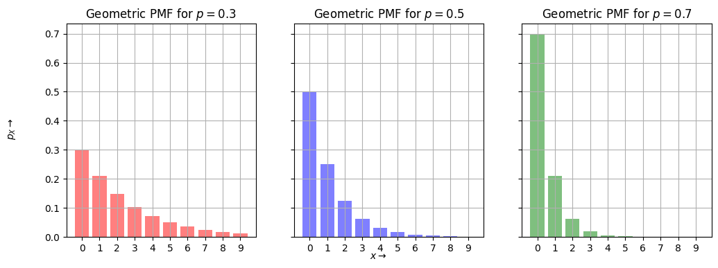
../_images/5a2fc194efed4ee5845c7bb9466c20859ce70398b4b0612fd4a11c457795acc1.png

Geometric Random Variable#

from scipy.stats import geom


n=10
x = np.arange(1,n+1,1)
xs = [str(x[i]-1) for i in range(len(x))]
p = [0.3,0.5,0.7]
width = 0.35  # the width of the bars
cols = ['r', 'b', 'g']
fig, axs = plt.subplots(1,len(p), figsize=(4*len(p),4), sharey=True)
for i in range(len(p)):
    axs[i].bar(xs, geom.pmf(x, p[i]), alpha=0.5, color=cols[i])
    axs[i].set_title('Geometric PMF for $p={}$'.format(p[i]))
    axs[i].grid()
fig.text(0.5, 0.04, r'$x\rightarrow$', ha='center', va='center')
fig.text(0.06, 0.5, r'$p_X\rightarrow$', ha='center', va='center', rotation='vertical')

plt.show()

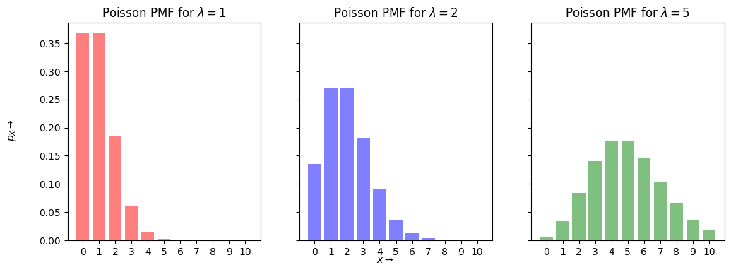
../_images/7458deac6cb7958bc6fcc17abaaccbb910796c41740b9e31ee24d5c3dc75a440.png

Poisson Random Variable#

from scipy.stats import poisson


n=10
x = np.arange(0,n+1,1)
xs = [str(x[i]) for i in range(len(x))]
param = [1,2,5]
width = 0.35  # the width of the bars
cols = ['r', 'b', 'g']
fig, axs = plt.subplots(1,len(param), figsize=(4*len(param),4), sharey=True)
for i in range(len(p)):
    axs[i].bar(xs, poisson.pmf(x, param[i]), alpha=0.5, color=cols[i])
    axs[i].set_title('Poisson PMF for $\lambda={}$'.format(param[i]))

fig.text(0.5, 0.04, r'$x\rightarrow$', ha='center', va='center')
fig.text(0.06, 0.5, r'$p_X\rightarrow$', ha='center', va='center', rotation='vertical')

plt.show()

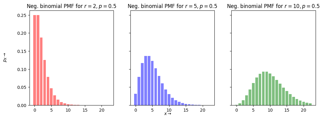
../_images/8bdecc4011a86565452dc490c4d7215ae84e1883790aa55e4fdfef29078b4bc5.png

Negative Binomial Random Variable#

from scipy.stats import nbinom

r = np.array([2, 5, 10])
p = 0.5
cols = ['r', 'b', 'g']
fig, ax = plt.subplots(1,len(r),figsize=(4*len(r),4), sharey=True)
x = np.arange(nbinom.ppf(0.01, r, p).min(), nbinom.ppf(0.99, r, p).max())
for i in range(len(r)):
    rv = nbinom(r[i], p)
    ax[i].bar(x, rv.pmf(x), alpha=0.5, color=cols[i])
    ax[i].set_title('Neg. binomial PMF for $r={}, p={}$'.format(r[i], p))

fig.text(0.5, 0.04, r'$x\rightarrow$', ha='center', va='center')
fig.text(0.06, 0.5, r'$p_X\rightarrow$', ha='center', va='center', rotation='vertical')

plt.show()

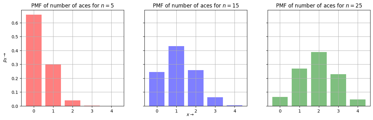
../_images/fb92af8dac741c94cab754b317dc898a59d2bc2532737328b7aba7f2b4f8d3aa.png

Hypergeometric Random Variable#

from scipy.stats import hypergeom


N, m = 52, 4
n = [5, 15, 25]
x = np.arange(0, m+1)

cols = ['r', 'b', 'g']
fig, ax = plt.subplots(1,len(n),figsize=(4.8*len(n),4), sharey=True)

for i in range(len(n)):
    rv = hypergeom(N, m, n[i])
    ax[i].bar(x, rv.pmf(x), alpha=0.5, color=cols[i])
    ax[i].set_title('PMF of number of aces for $n={}$'.format(int(n[i])))
    ax[i].grid()

fig.text(0.5, 0.04, r'$x\rightarrow$', ha='center', va='center')
fig.text(0.09, 0.5, r'$p_X\rightarrow$', ha='center', va='center', rotation='vertical')

plt.show()

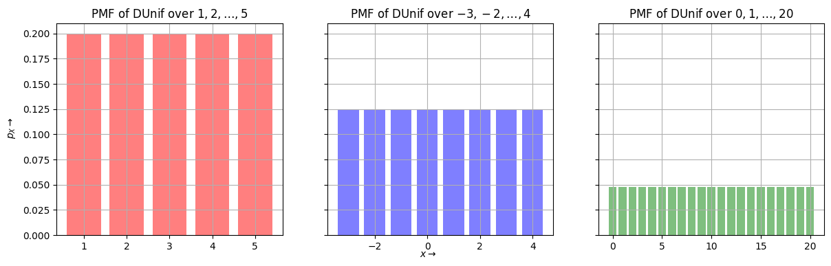
../_images/4b408bcb20477b667bb80f251cd13c75811efe5524b400cd492a245b8009f3b6.png

Discrete Uniform Random Variable#

from scipy.stats import randint


low = [1,-3,0]
high = [6,5,21]

cols = ['r', 'b', 'g']
fig, ax = plt.subplots(1,len(low),figsize=(4.8*len(low),4), sharey=True)

for i in range(len(low)):
    rv = randint(low[i], high[i])
    x = np.arange(low[i], high[i])
    ax[i].bar(x, rv.pmf(x), alpha=0.5, color=cols[i])
    ax[i].set_title('PMF of DUnif over ${},{},\ldots, {}$'.format(x.min(),x.min()+1, x.max()))
    ax[i].grid()

fig.text(0.5, 0.04, r'$x\rightarrow$', ha='center', va='center')
fig.text(0.08, 0.5, r'$p_X\rightarrow$', ha='center', va='center', rotation='vertical')

plt.show()

../_images/a46a43482f15ffea98890d61a0c80f336569b49c6468536fa871344c269990fc.png

Continuous Random Variables#

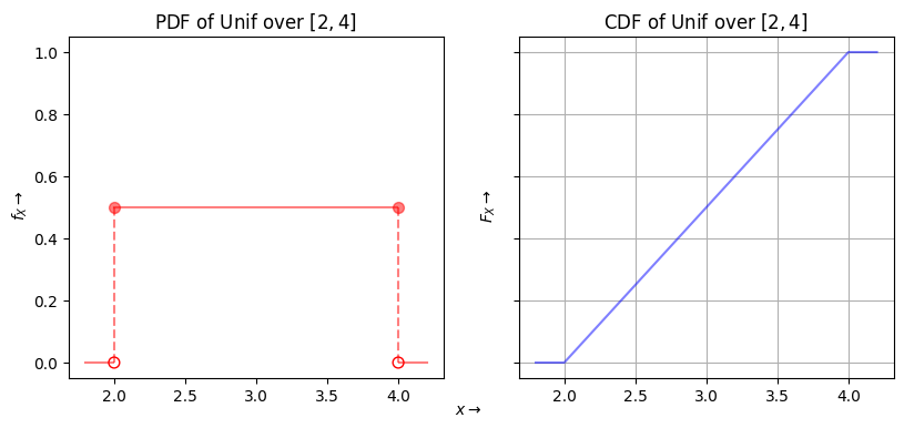
Uniform Random Variable#

from scipy.stats import uniform

fig, ax = plt.subplots(1,2,figsize=(4.8*2,4), sharey=True)

a = 2
b = 4
rv = uniform(a, b-a)
x = np.arange(a, b, 0.01)
ax[0].plot(x, rv.pdf(x), alpha=0.5, color=cols[0])
ax[0].set_title('PDF of Unif over $[{},{}]$'.format(a,b))
x = np.arange(a-0.2, a, 0.01)
ax[0].plot(x, rv.pdf(x), alpha=0.5, color=cols[0])
x = np.arange(b+0.01, b+0.2, 0.01)
ax[0].plot(x, rv.pdf(x), alpha=0.5, color=cols[0])
ax[0].scatter([a,b], rv.pdf([a,b]), s=50, alpha=0.5, color=cols[0])
ax[0].scatter([a,b], rv.pdf([a-0.01,b+0.01]), s=50, facecolors='none', edgecolors='r')
ax[0].plot([a,a], rv.pdf([a-0.01,a]), '--', alpha=0.5, color=cols[0])
ax[0].plot([b,b], rv.pdf([b,b+0.01]), '--', alpha=0.5, color=cols[0])
x = np.arange(a-0.2, b+0.2, 0.01)

ax[1].plot(x, rv.cdf(x), alpha=0.5, color=cols[1])
ax[1].set_title('CDF of Unif over $[{},{}]$'.format(a,b))
ax[1].grid()

fig.text(0.5, 0.04, r'$x\rightarrow$', ha='center', va='center')
fig.text(0.08, 0.5, r'$f_X\rightarrow$', ha='center', va='center', rotation='vertical')
fig.text(0.52, 0.5, r'$F_X\rightarrow$', ha='center', va='center', rotation='vertical')
plt.show()

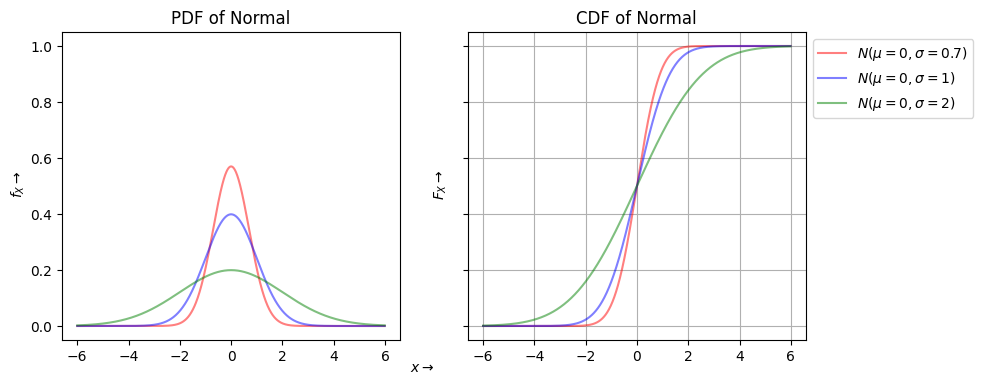
../_images/276441dc0c50be390e1418663065ab8919d1136cbed89d18eb87516b283bb08e.png

Normal Random Variable#

from scipy.stats import norm

fig, ax = plt.subplots(1,2,figsize=(4.8*2,4), sharey=True)

a = 0
b = [0.7,1,2]
x = np.arange(a-3*max(b), a+3*max(b), 0.01)
for i in range(len(b)):
    rv = norm(a, b[i])
    ax[0].plot(x, rv.pdf(x), alpha=0.5, color=cols[i],label='$N(\mu={},\sigma={})$'.format(a,b[i]))
    ax[1].plot(x, rv.cdf(x), alpha=0.5, color=cols[i])
ax[0].set_title('PDF of Normal')
ax[1].set_title('CDF of Normal')
ax[1].grid()
ax[0].legend(bbox_to_anchor=(2.2, 1.0), loc='upper left')

fig.text(0.5, 0.04, r'$x\rightarrow$', ha='center', va='center')
fig.text(0.08, 0.5, r'$f_X\rightarrow$', ha='center', va='center', rotation='vertical')
fig.text(0.52, 0.5, r'$F_X\rightarrow$', ha='center', va='center', rotation='vertical')
plt.show()

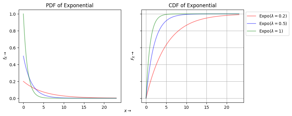
../_images/da7e8fa50b571c65c8b7964263f73978d1138633b9e18cce119e3ff475bee31a.png

Exponential Random Variable#

from scipy.stats import expon

la = [0.2,0.5,1]
x = np.arange(0, expon.ppf(0.99, scale = 1/min(la)), 0.01)

fig, ax = plt.subplots(1,2,figsize=(4.8*2,4), sharey=True)

for i in range(len(la)):
    rv = expon(scale = 1/la[i])
    ax[0].plot(x, rv.pdf(x), alpha=0.5, color=cols[i],label='Expo$(\lambda={})$'.format(la[i]))
    ax[1].plot(x, rv.cdf(x), alpha=0.5, color=cols[i])
ax[0].set_title('PDF of Exponential')
ax[1].set_title('CDF of Exponential')
ax[1].grid()
ax[0].legend(bbox_to_anchor=(2.2, 1.0), loc='upper left')

fig.text(0.5, 0.04, r'$x\rightarrow$', ha='center', va='center')
fig.text(0.08, 0.5, r'$f_X\rightarrow$', ha='center', va='center', rotation='vertical')
fig.text(0.52, 0.5, r'$F_X\rightarrow$', ha='center', va='center', rotation='vertical')
plt.show()

../_images/198f08c967087b30029ee884cb7b058df2b7e031b3bb930c9865d248e66b252d.png

from IPython.display import HTML
HTML('<iframe width="560" height="315" src="https://www.youtube.com/embed/LIN9PcfPoZg?rel=0&amp;controls=0&amp;showinfo=0" frameborder="0" allowfullscreen></iframe>')

/usr/share/miniconda3/envs/econschool-notebook/lib/python3.8/site-packages/IPython/core/display.py:431: UserWarning: Consider using IPython.display.IFrame instead
  warnings.warn("Consider using IPython.display.IFrame instead")

HTML('<iframe width="560" height="315" src="https://www.youtube.com/embed/FY3CTcQQ_i0?rel=0&amp;controls=0&amp;showinfo=0" frameborder="0" allowfullscreen></iframe>')